A Word from Ilya Sutskever (L01-3)
Early in the lecture there is a quote from Ilya Sutskever.
“Compute has been the oxygen of deep learning.”
He said it at the 50th anniversary event for the ACM Turing Award in 2017. Good algorithms alone run nothing. Compute has to back them up. I read this sentence as the shortest answer to why MLSys is needed.
Models keep changing. CNNs gave way to Transformers, and structures like MoE and Mamba are common now. Each shift shakes the model-side knowledge, but the problem of running models efficiently on real hardware does not go away. “AI-resistant career” sounds a bit grand, but I agree that MLSys is a field with staying power.
AI Ingredients: The Three Elements (L01-2)
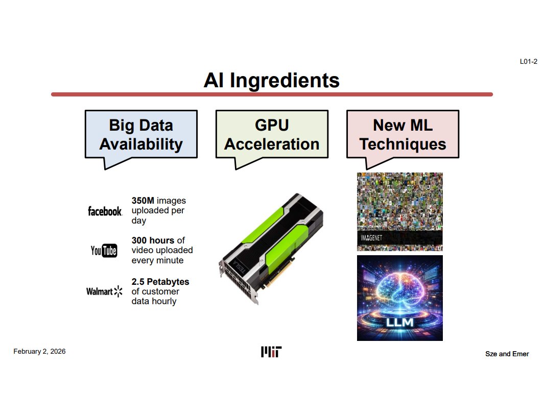
The lecture groups the ingredients of today’s AI into Big Data, GPU Acceleration, and New ML Techniques.
Big Data. Facebook receives 350 million images a day, YouTube accumulates 300 hours of video per minute, and Walmart processes 2.5PB of data per hour. Large-scale training became possible because this much data piled up for models to consume.
GPU Acceleration. GPUs like the Tesla T4 process matrix multiplications in massive parallel. They brought training workloads that CPUs could not handle into realistic time budgets.
New ML Techniques. AlexNet opened the CNN era and the Transformer created today’s LLMs. When the algorithm changes, the conditions for well-matched hardware change with it.
Remove any one of the three and AI at today’s scale would be hard to reach. This course digs into the compute side.
How GPUs Evolved for DNNs (L01-4)
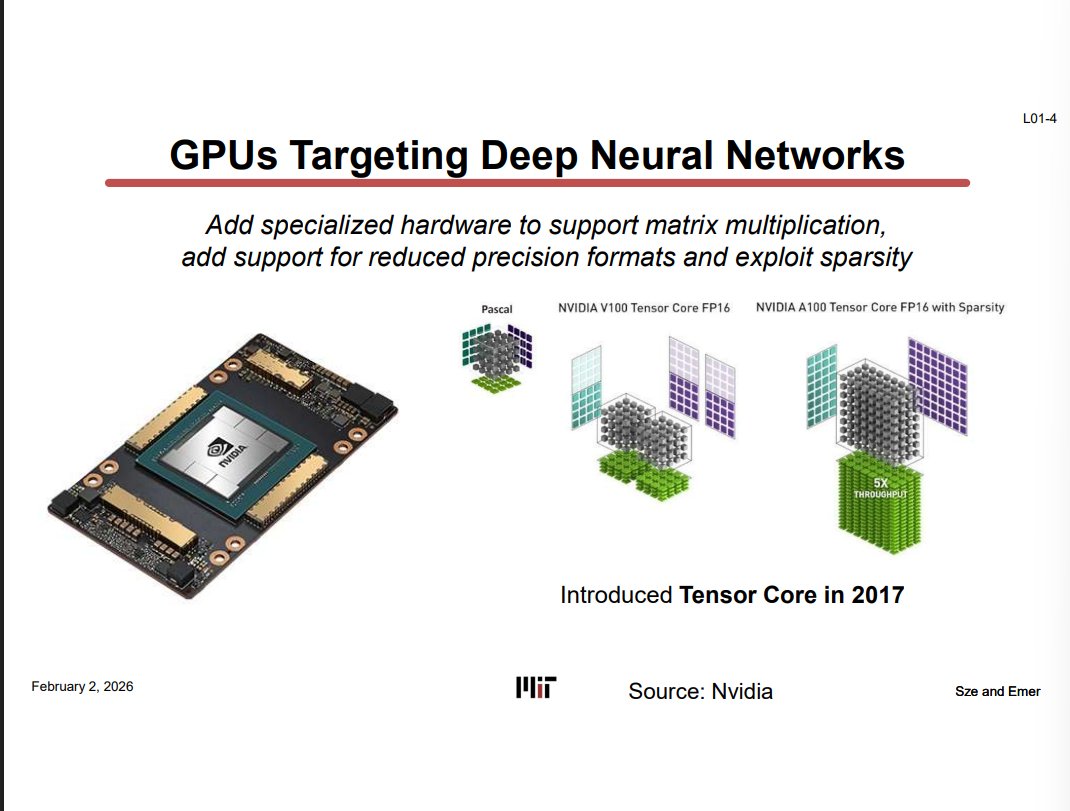
Up through Pascal, matrix multiplication was mostly handled by general-purpose CUDA cores. In 2017 the V100 added Tensor Cores. Instead of repeating scalar FMAs on CUDA cores, small-matrix multiply-accumulate runs on a dedicated unit. That raised DNN throughput per area substantially, and FP16 support added to the gain.
With the A100 in 2020, Tensor Cores began supporting 2:4 structured sparsity. If the pattern of two zeros out of every four consecutive elements is met, the zero terms are skipped and only the valid values are computed.
Not every sparse matrix gets faster here. The pruning result has to fit the 2:4 pattern the hardware understands. This is one place where it becomes clear that algorithms and hardware cannot be designed separately.
Software Companies Building Their Own HW (L01-5)
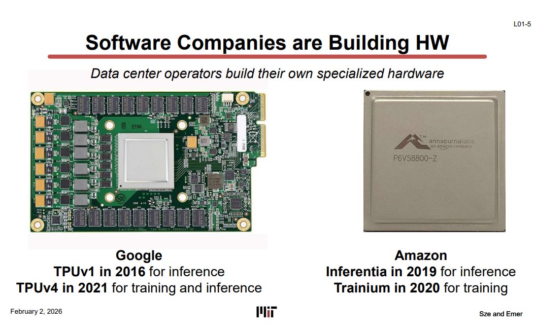
Google and Amazon buy NVIDIA GPUs in volume and also build their own chips. The reasons are cost and optimization.
A GPU is a general-purpose device that has to serve everything from graphics to scientific computing. If the datacenter workload narrows down to DNN inference and training, a chip built for just those operations can win on power and area.
Google’s TPU v1 came out for inference and used a 256×256 systolic array. From v2 it supported training as well. Amazon built Inferentia and Trainium to lower inference and training costs on AWS. In Korea, FuriosaAI and Rebellions are attacking the same problem in their own ways.
Cerebras WSE (L01-6)
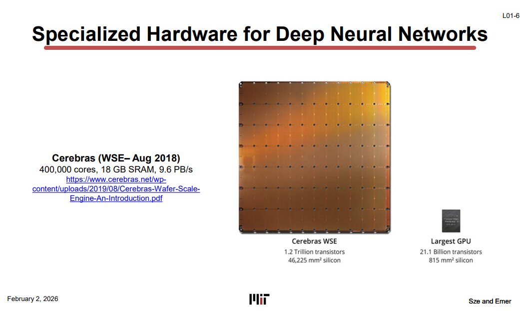
Cerebras WSE is the case that pushes this direction to the limit. Normal chips are small dies cut from a wafer; Cerebras uses the entire wafer as one chip. That gives it 18GB of on-chip SRAM. Considering that A100 on-chip SRAM is around 20MB and TPUs stay under 32MB, the scale is different.
It is not free, of course. Yield, cooling, and price problems follow. It is less a widely used answer than a design that shows how bold you can get for a specific workload.
Mobile SoCs for DNNs (L01-7)
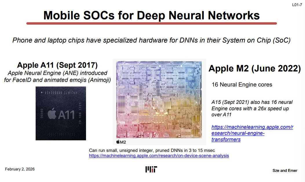
DNN-specific units are not only in datacenters. They are already in phones and laptops.
Apple’s A11 first shipped a 2-core ANE in 2017, mainly for on-device inference like Face ID and Animoji. The M2’s ANE in 2022 has 16 cores. The 26x performance gain over A11 includes both the core count increase and per-generation architecture improvements.
On mobile, model size, integer quantization, and prunability matter in particular, because power and memory cannot be spent as freely as on a server.
Rising Energy Consumption of Computing (L01-8)
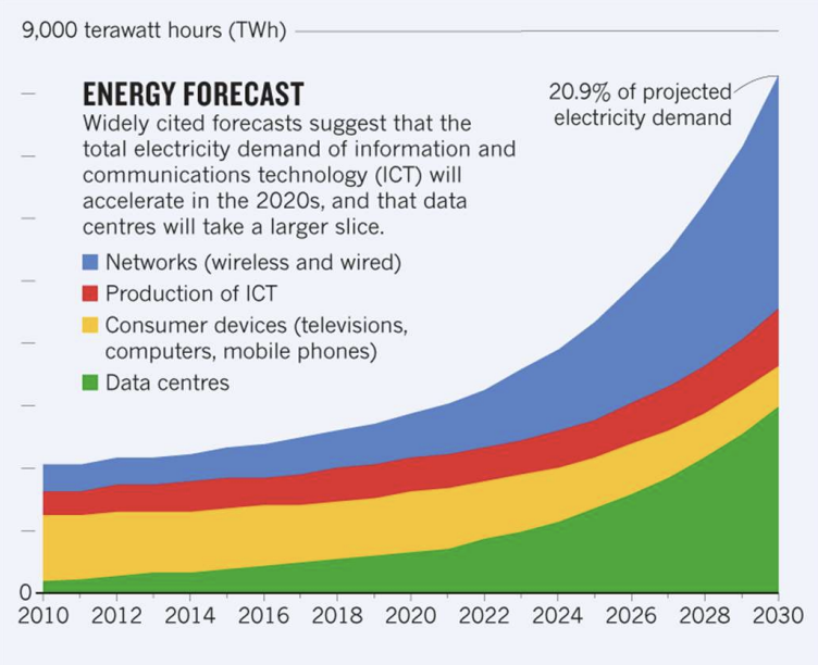
The slide cites a 2024 Goldman Sachs projection that US datacenters’ share of electricity could grow from 3% in 2022 to 8% by 2030, along with a forecast that ICT as a whole could account for 20.9% of global electricity.
Models keep growing and power is not unlimited. That is how finishing the same computation with less energy became a systems problem.
What matters here is that data movement costs more than the computation itself. In the slide’s 65nm numbers, one DRAM access consumes about 200x the energy of an ALU operation. Making the arithmetic units faster is not enough. The number of long-distance data trips has to come down first.
That is why Cerebras made its on-chip SRAM huge. Ordinary accelerators follow the same principle with a memory hierarchy of register file, local buffer, global buffer, and DRAM, reusing data from the near end as much as possible.
Computing Cost of ChatGPT (L01-12)
GPT-3 has 96 layers and 175B parameters. Training is put at a total of 3.14×10²³ FLOPs.
By the slide’s arithmetic, that takes 355 years on a single V100 and costs about $4.6M in cloud compute, roughly 6 billion KRW. GPT-4's training cost is estimated at over $100M.
The exact range matters less than the scale. Each generation of model growth pushed the compute cost up at a pace that is hard to absorb.
Changing Trends: DeepSeek (L01-13)
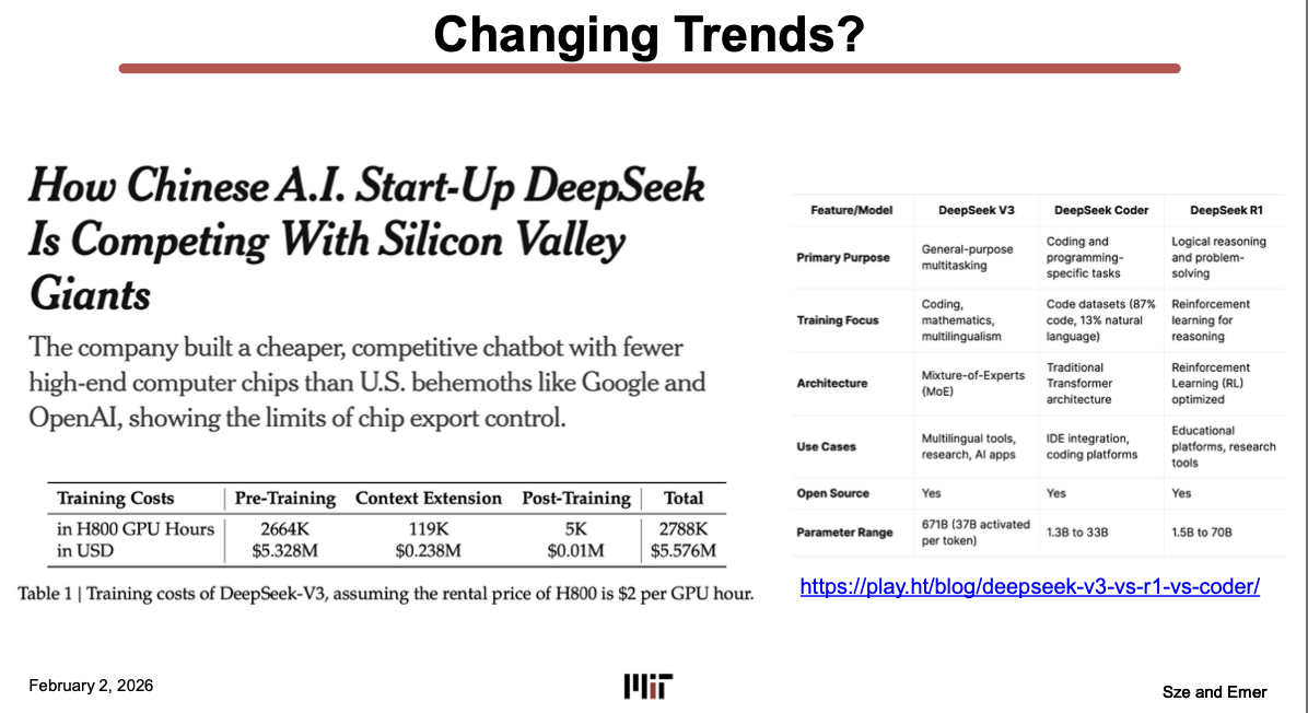
The slide puts GPT-4’s estimated training cost next to DeepSeek’s published figure: over 130 billion KRW for GPT-4 versus about 8 billion KRW for DeepSeek.
The two are not the same line item, though. The DeepSeek number is close to the GPU rental cost of the final training run, while the GPT-4 number is a much broader total cost estimate. Dividing one by the other and calling it several times cheaper breaks the comparison.
What stands out in DeepSeek’s architecture is MoE. Total parameters are 671B, but only 37B activate per token. Instead of running every expert every time, it picks the necessary subset and cuts the computation.
Training vs Inference (L01-15)
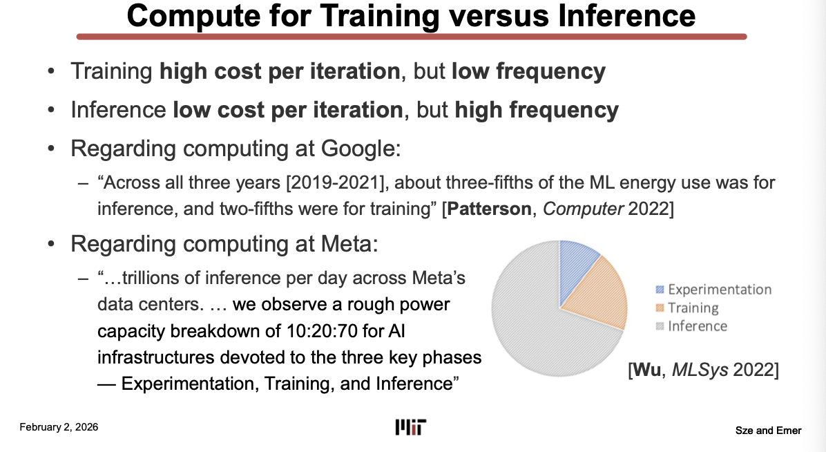
Training costs a lot per run, but per model it runs few times. Inference costs relatively little per call and keeps getting called for as long as the service is alive.
Sending one question to a chatbot and getting an answer is one inference. When such requests pile up to trillions per day, the cumulative cost becomes a bigger problem than training. This is also why LLM inference optimization exists as its own job category.
Why On-Device (L01-18)
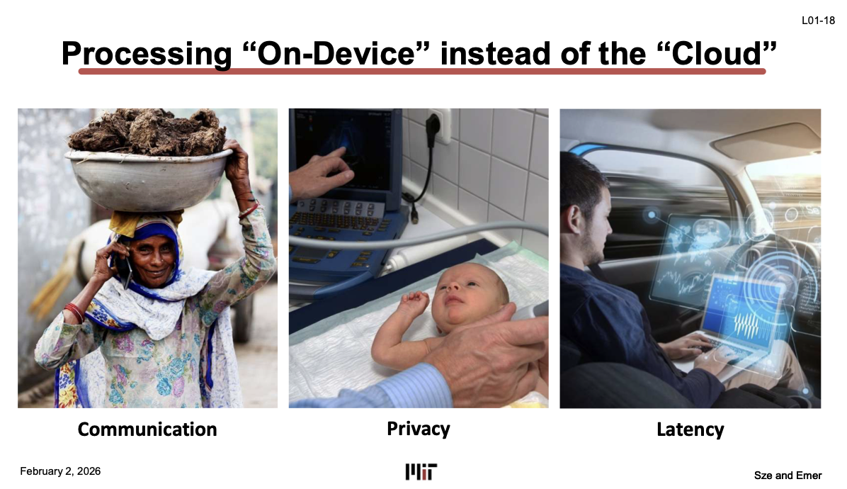
There are three reasons to run inference on the device instead of the cloud.
Communication. Where the network is absent or unstable, a cloud model cannot be called.
Privacy. Data that should not leave, like medical records or defense data, is safer processed on the device.
Latency. In systems that must react immediately, like autonomous driving, tens to hundreds of milliseconds of round trip can be fatal.
Self-Driving Cars (L01-19)
Autonomous driving is an example where the demands of edge inference show up all at once.
Cameras and radar generate about 6GB of data every 30 seconds. Assume one car runs 10 DNNs at 60Hz over 10 cameras: that is 21.6M inferences per hour. With a million vehicles, 21.6 trillion per hour.
When a prototype compute rig draws 2,500W, air cooling barely holds. Sending all the sensor data to the cloud is not an option either; the traffic and latency turn directly into safety problems.
The Slowing of Moore’s Law and the Need for Domain-Specific HW (L01-22)
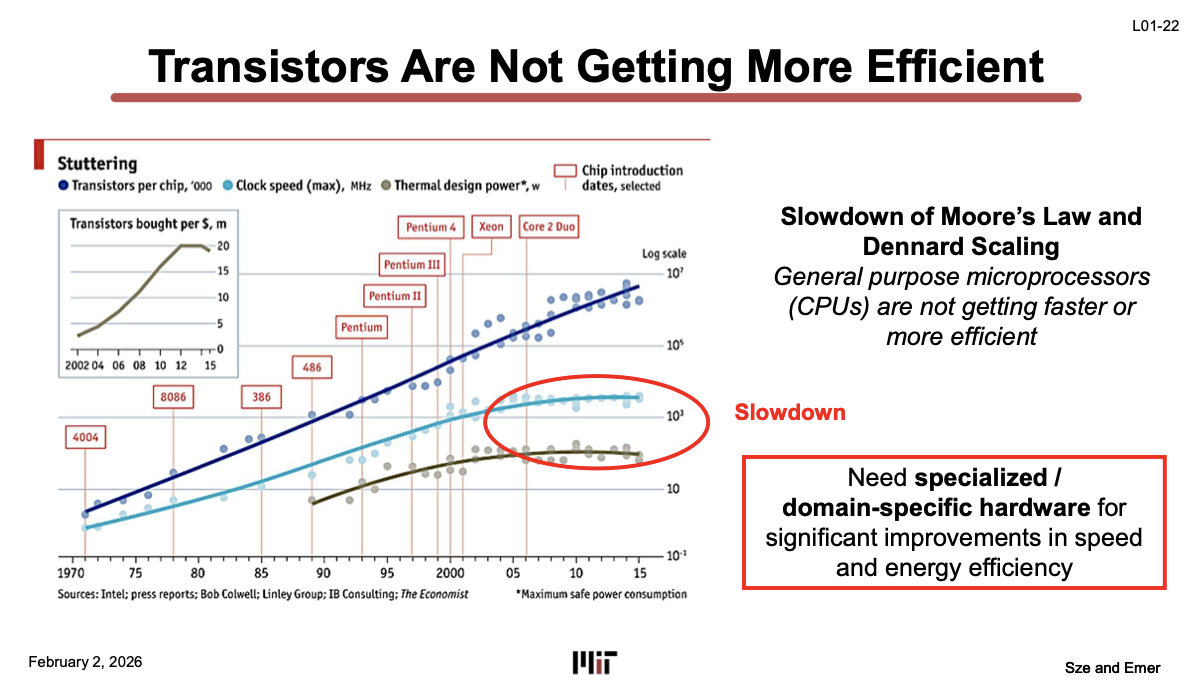
Behind MLSys becoming its own field are the slowdowns of Moore’s Law and Dennard Scaling.
Transistor counts still grow, but not at the old rate. Transistors per dollar are stagnating too. Dennard Scaling, where power shrank along with transistor size, broke around 2005. That is why clock speed and TDP no longer climb much in the slide.
Since general-purpose processor performance and efficiency no longer improve automatically with a new process, hardware matched to specific operations became necessary. Tensor Cores focus on matrix multiplication, Google TPUs on DNN training and inference, Apple ANE on on-device inference, and FuriosaAI NPUs on AI inference.
L01-23 to L01-25: The Evolution of the CPU Pipeline
This part shows how much control logic a general-purpose CPU carries to achieve high utilization. For regular matrix computations like DNNs, that complexity does not turn into gains.
Simple In-Order Pipeline (L01-23)
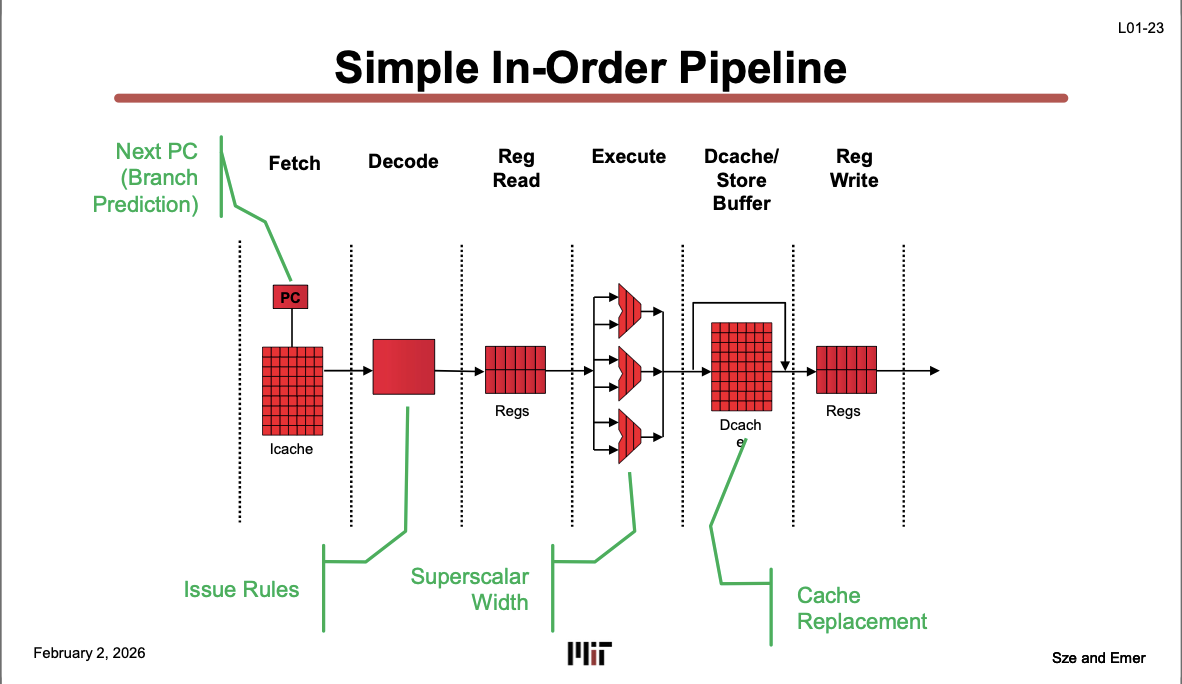
The pipeline on the slide is a 6-stage version of the IF, ID, EX, MEM, WB structure, with ID split into Decode and Reg Read. Doing less per stage leaves room to raise the clock. It handles multiple instructions per cycle, so it is also superscalar.
Fetch reads the instruction at the PC’s address from the I-cache. The next PC is chosen by the branch predictor.
Decode interprets the opcode, rs, rd, and immediate. Reg Read pulls the needed operands from the register file.
Execute is where the ALU does the actual work. Three red chevrons in the figure mean three functional units usable at once. Think of a combination like an integer ALU, an FP or multiply unit, and a branch unit.
The D-cache and store buffer handle loads and stores, and Reg Write puts results back into the register file.
Basic Out-of-Order Pipeline (L01-24)
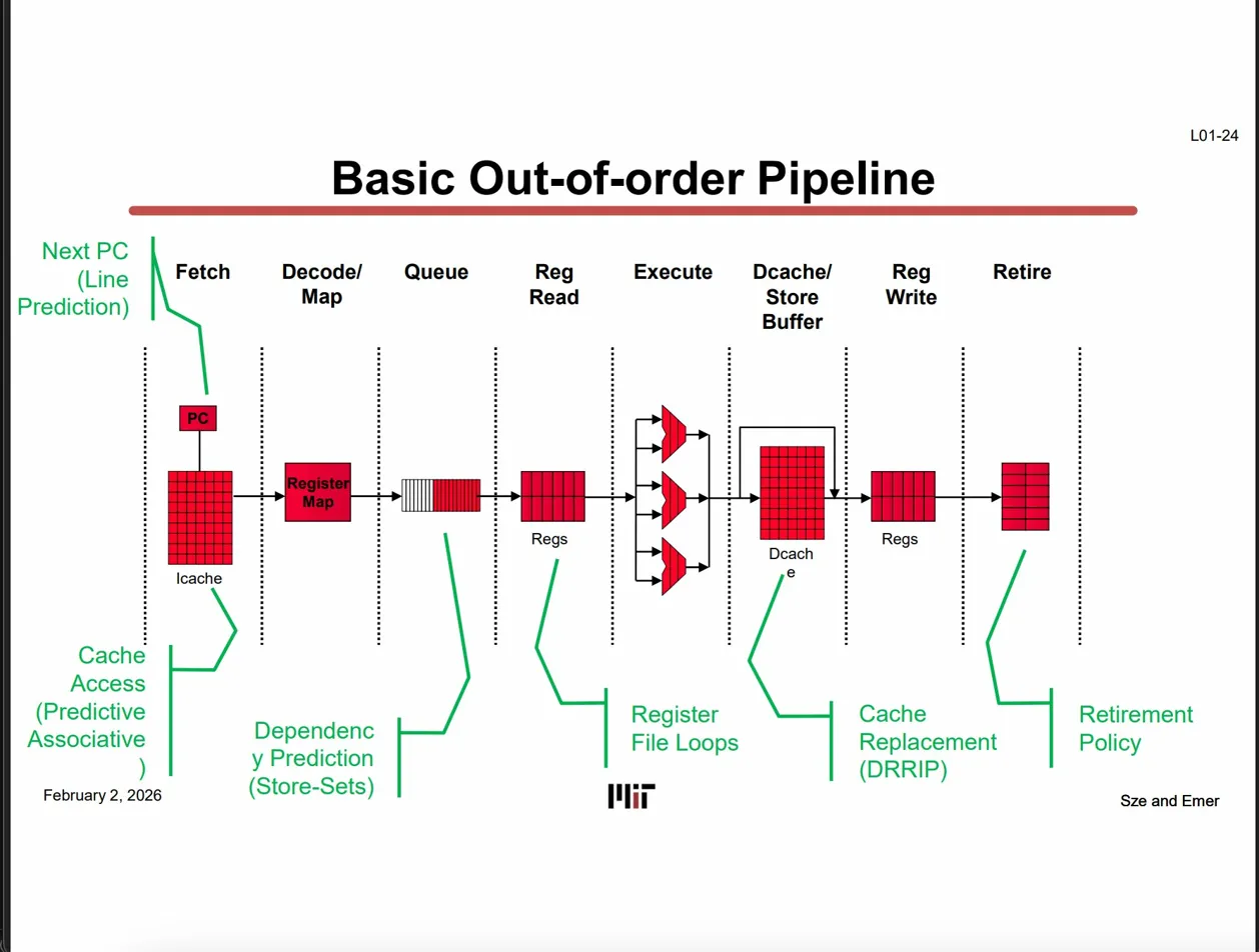
An in-order superscalar stalls everything behind an instruction that hits a cache miss, even if later instructions are ready. Three functional units sit idle if work does not arrive.
An out-of-order design adds an issue queue and sends whichever instructions have their operands ready. While an earlier load waits on memory, independent later instructions fill the empty slots.
SMT: Simultaneous Multi-Threading (L01-25)
SMT here is a different concept from the GPU’s SIMT.
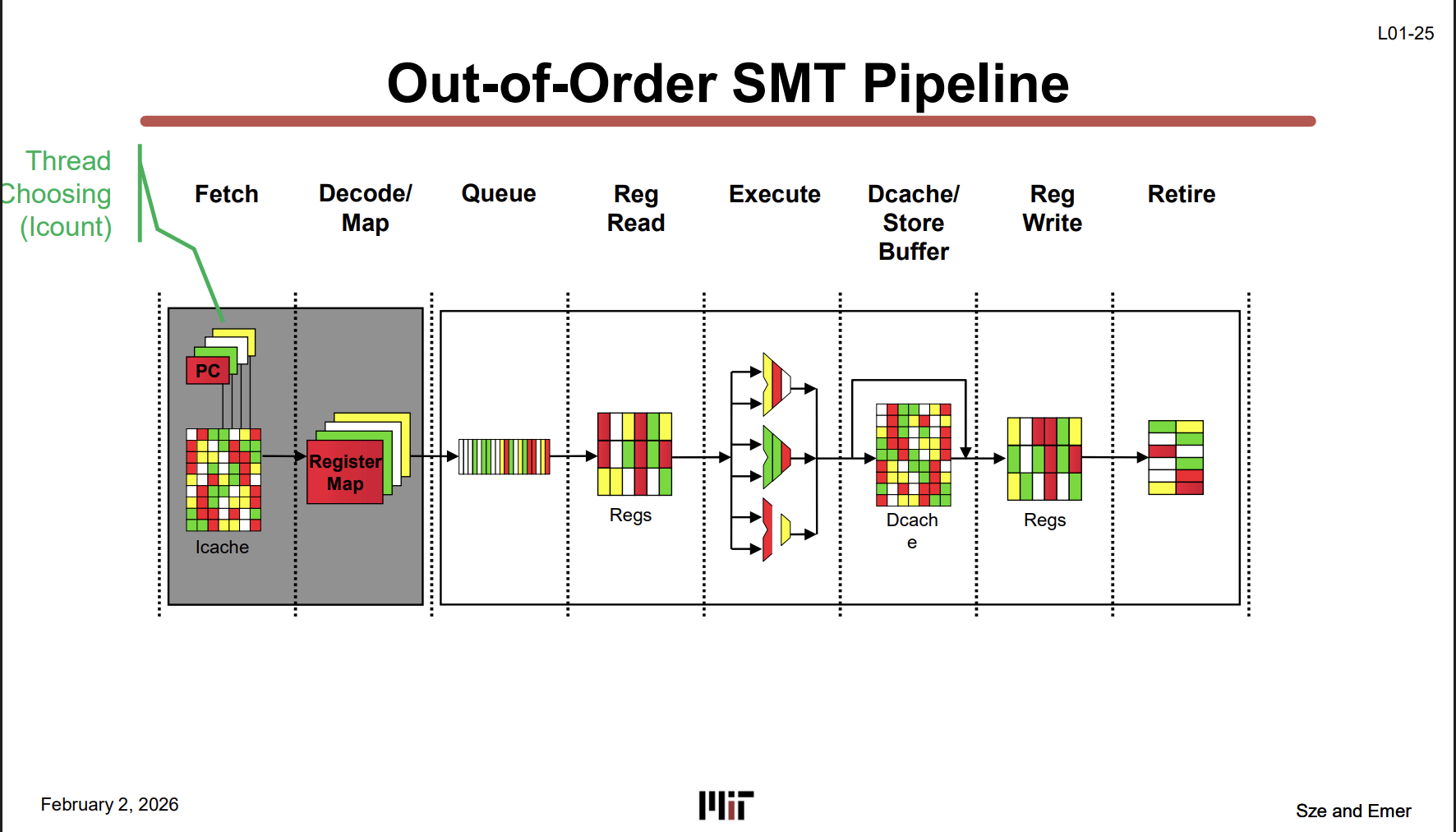
The red, yellow, and green in the figure are different threads. The pipeline is not replicated per thread; multiple threads share one pipeline. Intel famously worked this to great effect under the name Hyper-Threading.
When one thread stalls, ready instructions from another thread fill the empty slots and raise throughput.
| Structure | Characteristics |
|---|---|
| Scalar | 5-stage, width=1, one instruction per cycle |
| Superscalar (In-Order) | width>1, several per cycle, in order |
| OoO + Superscalar | width>1, ready instructions go first |
| OoO + SMT | multiple threads share one pipeline |
Branch prediction, register renaming, the issue queue, retire, thread choosing: all of it is control logic added for generality. For the repetitive MatMuls of DNNs this complexity is overkill. That is why accelerators lead with a PE array and a memory hierarchy instead of a complex CPU pipeline.
Accelerator Diversity (L01-26)
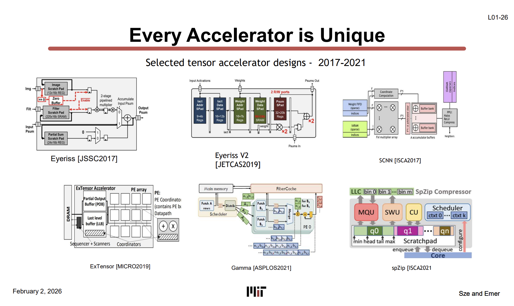
Not all DNN accelerators look alike. When the target workload changes, PE placement, memory hierarchy, and dataflow change too.
Eyeriss is a spatial array for CNN inference with a local scratchpad in each PE.
Eyeriss V2 added a more flexible NoC.
SCNN focuses on skipping zeros in sparse CNNs.
ExTensor and Gamma target sparse tensor and sparse matrix computation respectively.
spZip handles compression and decompression of sparse data.
CPU pipelines are fairly standardized in their broad structure. Accelerators diverge from the design stage depending on dense versus sparse, CNN versus Transformer. Analyzing these differences in a common language is the main body of the course.
PE stands for Processing Element. It is a small compute unit close to a CPU’s ALU, usually a multiplier, an adder, and a small register file bundled to handle MACs.
TeAAL Pyramid of Concerns & FuseMax (L01-28 to L01-34)
The vocabulary suddenly thickens here. In the first lecture, rather than memorizing every name, it is enough to pick up the sense of splitting things into layers.
TeAAL Pyramid of Concerns (L01-28)
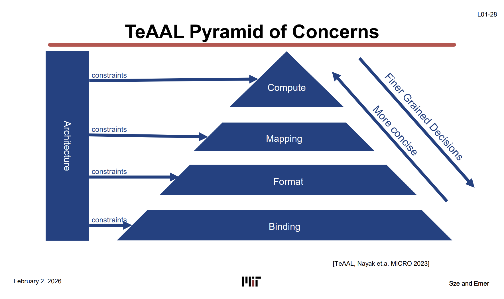
TeAAL splits accelerator design into four layers. Decisions get finer toward the top, and the architecture constrains what each layer can do.
| Layer | Meaning | Course link |
|---|---|---|
| Compute | What operation runs. MatMul, Attention, etc. | Lab 1: Einsum |
| Mapping | How the operation is placed on hardware. Tiling, dataflow, etc. | Lab 2, 3 |
| Format | How data is stored. Dense, sparse, etc. | Lab 4: Sparsity |
| Binding | How operations and data are assigned to actual PEs and buffers | Lab 2, 3 |
Most of the design problems later in the course can be placed back into these four boxes.
FuseMax: The Pyramid Applied (L01-29)
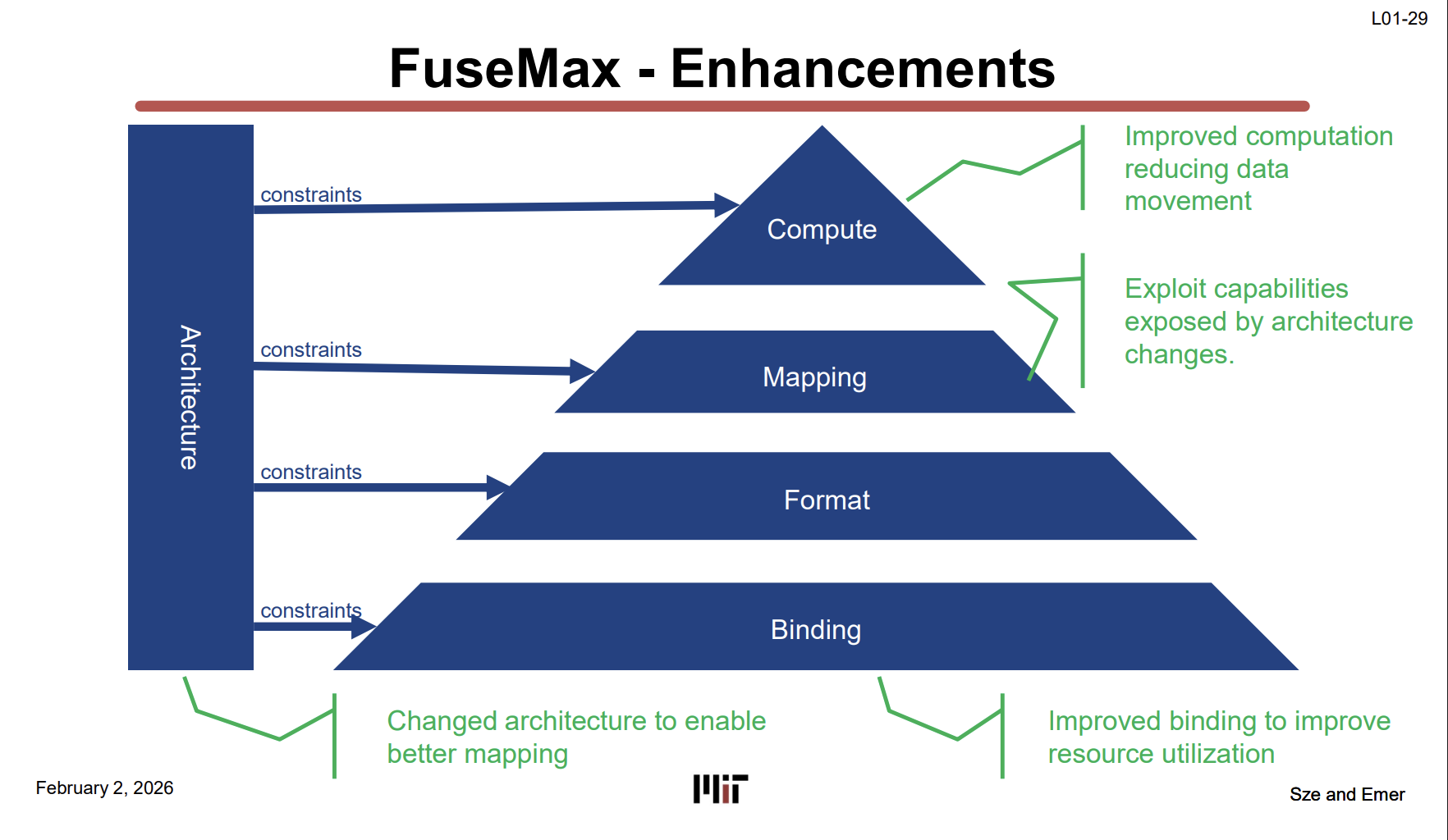
FuseMax is a design that accelerates Transformer attention. Reworking compute, mapping, and binding in turn, it lifts a low PE utilization to about 90%.
| Step | Layer | Change | Result |
|---|---|---|---|
| Cascade | Compute | Fuse MatMul and Softmax to cut intermediate data movement | small utilization gain |
| Architecture change | Architecture and Mapping | Change the structure so a new mapping becomes possible | further gain |
| Binding improvement | Binding | Distribute work more evenly across PEs | about 90% utilization |
Unfused runs Q×K, Softmax, and ×V separately, writing intermediate results to memory at each step. FLAT is the existing partial fusion approach. Cascade binds the stages more tightly so intermediates never leave for memory.
No single step delivers the performance alone. How the operations are fused, the hardware structure, and the actual resource assignment have to line up together.
PE Utilization Across the Steps (L01-30 to L01-34)
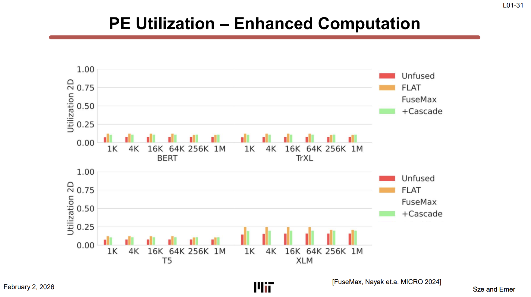
In the L01-30 baseline, BERT, TrXL, T5, and XLM all sit below 0.25 PE utilization from sequence length 1K to 1M. Hundreds of PEs are built and mostly idle.
The x-axis is sequence length, the y-axis PE utilization. Red Unfused and orange FLAT both stay low. Applying Cascade, Architecture, and Binding in turn from L01-31 to L01-33 raises utilization to about 90%.
The Basic Structure of a DNN Accelerator (L01-43)
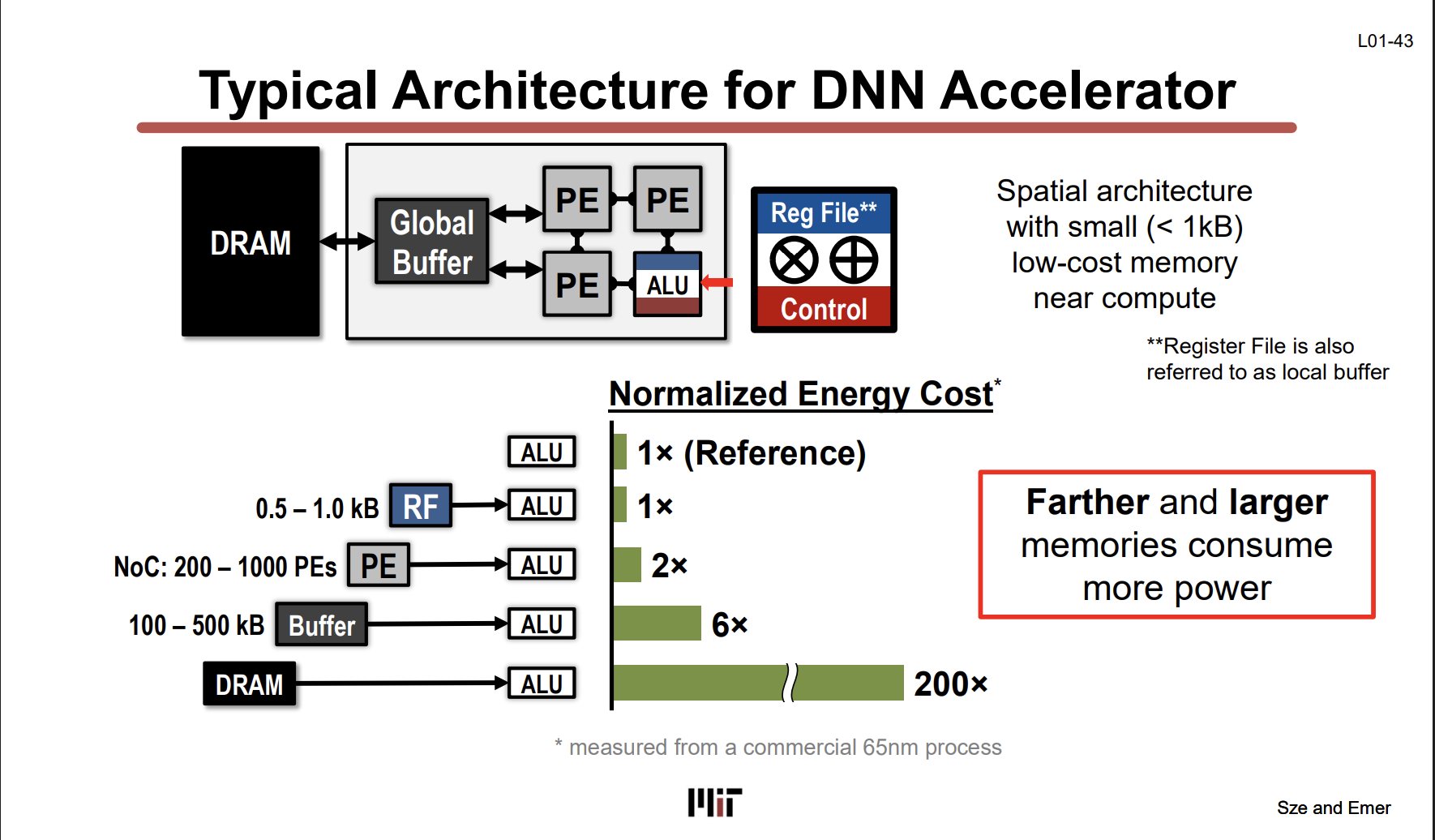
A typical DNN accelerator has a PE array and a memory hierarchy instead of a complex CPU pipeline.
Data comes from DRAM into a Global Buffer and on to the PE array. Each PE holds a Reg File smaller than 1kB, an ALU, and simple control. PE counts run from hundreds to thousands, and the Global Buffer is roughly 100kB to 500kB.
Each PE concentrates on simple, repetitive operations like MAC. With no area spent on branch prediction or register renaming, more compute units fit in the same chip area.
The slide’s normalized energy cost at 65nm:
| Where the data comes from | Energy cost |
|---|---|
| The ALU operation itself | 1× |
| Reg File to ALU | 1× |
| Inter-PE NoC to ALU | 2× |
| Global Buffer to ALU | 6× |
| DRAM to ALU | 200× |
One DRAM access costs 200x the actual computation. The same table explains why Cerebras put in 18GB of SRAM.
“Farther and larger memories consume more power.”
Keep this sentence in mind and the dataflow and tiling discussion later in the course reads much more easily.
Accelerator Design Decisions (L01-44)
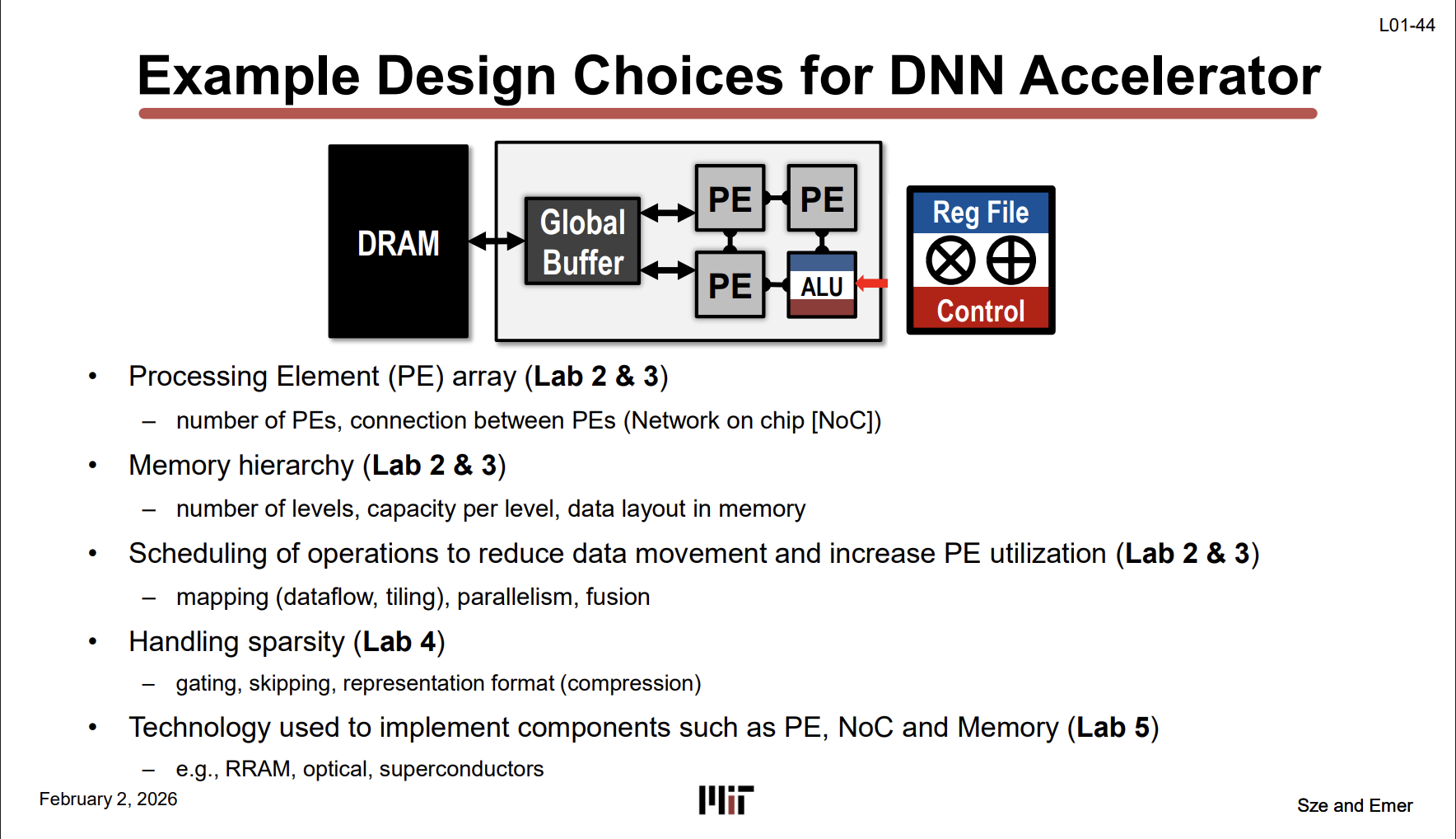
The items a designer has to choose connect to the course Labs.
| Design decision | Details | Lab |
|---|---|---|
| PE array | Number of PEs and how they connect | Lab 2, 3 |
| Memory hierarchy | Number of levels, capacity, data placement | Lab 2, 3 |
| Scheduling | Mapping, dataflow, tiling, parallelism, fusion | Lab 2, 3 |
| Sparsity handling | Gating, skipping, compression formats | Lab 4 |
| Implementation technology | RRAM, optical, superconductors, etc. | Lab 5 |
TeAAL’s Compute, Mapping, Format, and Binding come down to actual design variables here.
Roofline-Based Inefficiency Analysis (L01-45)
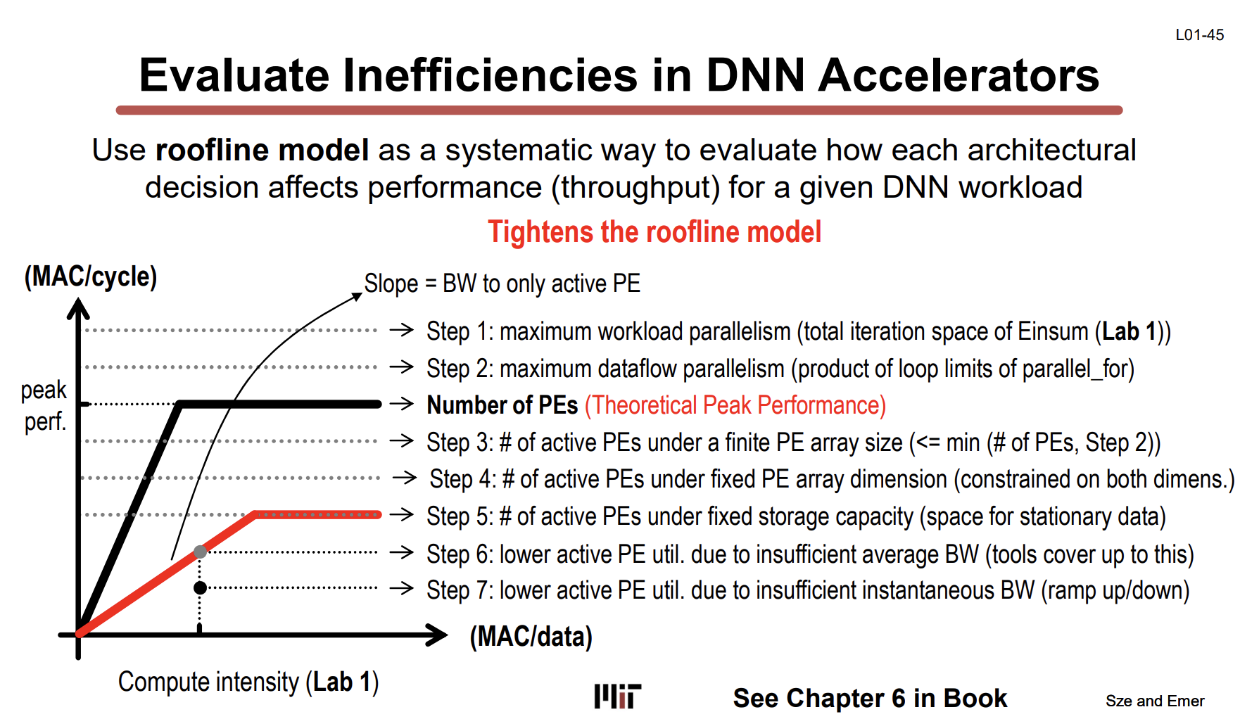
The Roofline Model is a frame for seeing whether performance is blocked by computation or by memory bandwidth. The x-axis is compute intensity, the y-axis performance. A larger x value means more operations per piece of data fetched. The sloped line is the limit set by memory bandwidth; the flat line on the right is the limit set by compute peak.
Stuck to the left slope means memory-bound; stuck to the right plateau means compute-bound.
Steps 1 through 7 on the slide show how much the theoretical peak gets shaved as it meets real constraints.
| Step | Constraint | Lab |
|---|---|---|
| Step 1 | Maximum parallelism in the workload itself | Lab 1 |
| Step 2 | Maximum parallelism the dataflow allows | Lab 2, 3 |
| PE count | The hardware’s theoretical peak | none |
| Step 3 | Finite PE array size | Lab 2, 3 |
| Step 4 | PE array dimension constraints | Lab 2, 3 |
| Step 5 | Finite storage capacity | Lab 2, 3 |
| Step 6 | Insufficient average bandwidth | Lab 2, 3 |
| Step 7 | Insufficient instantaneous bandwidth | none |
Each constraint added tightens the roofline downward. Instead of stamping actual performance as a single number from the start, you can separate out where and how much got shaved.