Signals and Systems

Reference: Samir S. Soliman, Mandyam D. Srinath, Continuous and Discrete Signals and Systems, 2nd ed., Prentice Hall, 1998. Chapter 1, Representing Signals.

This course covers continuous-time signals with a single independent variable, time, and leaves discrete-time signals to the DSP¹ course. The material below corresponds to Sections 1.1 through 1.3 of the textbook and to lecture slides² 2 through 9.

Definition of a signal

A signal is a detectable physical quantity that carries information. The definition has three parts.

1. It is a physical quantity or a variable that represents one. The amplitude of a voice, the brightness of a screen pixel, and the current in a circuit all qualify.
2. It is detectable³. The receiving side must be able to measure the quantity.
3. It carries information. A quantity that can be detected but carries no information is not treated as a signal.

Mathematically a signal is written as a function of one or more independent variables (the inputs of the function). The number of independent variables⁴ depends on the signal.

Signal	Notation	Independent variables
Voice, circuit current $i(t)$, voltage $v(t)$	$A(t)$	Time $t$ only
Image	$p(x, y)$	Two coordinates $x, y$
Electric field	$E(x, y, z, t)$	Three spatial coordinates and time

This course deals only with signals $x(t)$ whose single independent variable is time $t$. An image $p(x, y)$ belongs to an image processing course, and a video is $p(x, y, t)$ with time added.

Continuous-time and discrete-time signals

A continuous-time signal is a signal whose independent variable is defined over an entire interval of real numbers. In the definition, the word continuous modifies the independent variable, not the function value⁵. For a radio signal $v(t)$ the independent variable is time $t$, and for atmospheric pressure $p(h)$ it is altitude $h$. Both independent variables sweep the whole real line, so both are continuous-time signals. An independent variable other than time, such as altitude, falls in the same class as long as it is continuous.

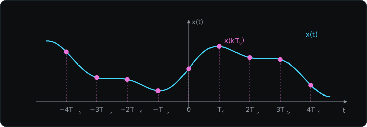
A discrete-time signal is a signal whose independent variable takes only discrete values. Taking the values of a continuous-time signal $x(t)$ only at $t = kT_s$ gives $x(kT_s)$. $T_s$⁶ is a fixed positive real number and $k$ is an integer ($0, \pm 1, \pm 2, \dots$). With $T_s = 2$ the signal is defined only at $t = 0, \pm 2, \pm 4, \dots$. In the figure below the cyan curve is $x(t)$, which has a value at every real $t$, and the magenta dots are $x(kT_s)$, which has values only at $t = kT_s$. To tell the two apart, look at where the points sit on the $t$ axis rather than at the height of the function values.

Continuity of a function

A signal is a function, so the continuity of a signal follows the continuity of a function. $x(t)$ is continuous at $t = t_1$ when two conditions hold in order.

1. The left-hand limit $x(t_1^-)$ and the right-hand limit $x(t_1^+)$ are equal. The limit at $t_1$ then exists.
2. That limit equals the function value $x(t_1)$.

A signal continuous at every $t$ is a continuous signal. A signal with a finite number of discontinuities is piecewise continuous⁷. A signal with infinitely many discontinuities is not piecewise continuous.

Value at a discontinuity

Ordinary mathematics leaves the function value at a discontinuity undefined. This textbook defines the value at a discontinuity $t_1$ as the average⁸ of the left-hand and right-hand limits.

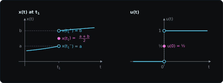
$$ x(t_1) = \frac{1}{2}\left[x(t_1^+) + x(t_1^-)\right] $$

The unit step function $u(t)$ is 0 for $t < 0$ and 1 for $t > 0$. At $t = 0$ the left-hand limit 0 and the right-hand limit 1 differ, so the limit does not exist, and the signal is piecewise continuous rather than continuous. Applying the average definition gives $u(0) = \tfrac{1}{2}$. In the left panel of the figure below, the two open circles are the left-hand limit $a$ and the right-hand limit $b$, and the filled dot is the value $\tfrac{a + b}{2}$ defined by the textbook. Applying the same rule in the right panel with $a = 0$ and $b = 1$ gives $u(0) = \tfrac{1}{2}$.

As an example, $x(t) = 2u(t - 1) - u(t - 3)$ is 0 for $t < 1$, 2 for $1 < t < 3$, and 1 for $t > 3$. The discontinuities are at $t = 1, 3$, with $x(1) = \tfrac{0 + 2}{2} = 1$ and $x(3) = \tfrac{2 + 1}{2} = \tfrac{3}{2}$. With two discontinuities the signal is piecewise continuous.

Rectangular pulse and pulse train

The rectangular pulse $\mathrm{rect}(t/\tau)$ is 1 for $|t| < \tfrac{\tau}{2}$ and 0 for $|t| > \tfrac{\tau}{2}$.

$$ \mathrm{rect}(t/\tau) = \begin{cases} 1, & |t| < \tau/2 \\ 0, & |t| > \tau/2 \end{cases} $$

The height is fixed at 1, and the parameter $\tau$⁹ sets the width of the base. The discontinuities are the two points $t = \pm\tfrac{\tau}{2}$, so the pulse is piecewise continuous, and since $t$ is defined over the whole real line it is a continuous-time signal.

Shifting $\mathrm{rect}(t/\tau)$ in time by a fixed spacing and adding the copies gives a pulse train¹⁰. A train of pulses of width 1 repeated every 2 units is written as follows, with $n$ ranging over all integers.

$$ x(t) = \sum_{n=-\infty}^{\infty} \mathrm{rect}(t - 2n) $$

The discontinuities at $t = 2n \pm \tfrac{1}{2}$ are infinite in number, so the train is neither continuous nor piecewise continuous. Since $t$ is defined over the whole real line, it is a continuous-time signal. Cutting the train to a finite number of pulses leaves a finite number of discontinuities, which makes it piecewise continuous.

Continuous versus continuous-time

The two terms describe properties on different axes.

Term	Axis	Criterion
continuous / piecewise continuous	Vertical axis (function value $x$)	Number of points where the limit conditions fail
continuous-time / discrete-time	Horizontal axis (independent variable $t$)	Whether $t$ is defined over a whole real interval or only at $t = kT_s$

Signal	Function-value property	Independent-variable property
$\sin t$	continuous	continuous-time
Rectangular pulse, $u(t)$	piecewise continuous	continuous-time
Infinite pulse train	Infinitely many discontinuities, not piecewise continuous	continuous-time
$x(kT_s)$	Function-value property not considered	discrete-time

However many discontinuities there are, a signal whose $t$ axis is the whole real line is a continuous-time signal. Every signal in this course is continuous-time, and the only question within that class is whether it is continuous or piecewise continuous.

Exercise 1

For $x(t) = 3\,\mathrm{rect}\!\left(\frac{t - 4}{2}\right)$, find the following.

(a) The interval of $t$ where the value is 3 (b) The discontinuities (c) The value at each discontinuity under the textbook definition (d) All integers $k$ for which $x(kT_s)$ is nonzero when sampled with $T_s = 1$

Solution. From the definition of $\mathrm{rect}(t/\tau)$, $\tau = 2$ and $t$ is replaced by $t - 4$, so the value is 3 where $|t - 4| < 1$, that is, for $3 < t < 5$. The discontinuities are at $t = 3, 5$. At both points the left-hand and right-hand limits are 0 and 3, so $x(3) = x(5) = \tfrac{0 + 3}{2} = \tfrac{3}{2}$. With $T_s = 1$ we have $t = k$, and the values at $k = 3, 4, 5$ are $\tfrac{3}{2}, 3, \tfrac{3}{2}$ respectively, with 0 at every other $k$.

Periodic signals and the fundamental period

A periodic signal is a continuous-time signal for which some positive $T$ satisfies the following at every $t$.

$$ x(t) = x(t + nT), \qquad n = 1, 2, 3, \dots $$

Because the condition must hold for every $t$, the signal is assumed to exist from $-\infty$ to $+\infty$¹¹. If $T$ is a period, then $2T$, $3T$, and $4T$ are periods as well. The smallest positive $T$ that satisfies the condition is the fundamental period¹², written $T_0$. A signal with fundamental period 2 also has 4 and 6 as periods. A signal with no such $T$ is aperiodic.

Sinusoids

A real-valued sinusoid is fixed by three parameters.

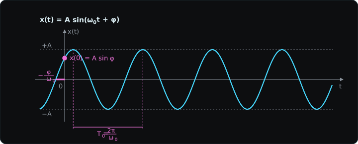
$$ x(t) = A\sin(\omega_0 t + \phi) $$

$A$ is the amplitude, and $x(t)$ stays between $-A$ and $A$. $\omega_0$ is the radian frequency in rad/s. $\phi$ is the initial phase¹³ in rad. The relation between radian frequency and frequency $f_0$ in Hz¹⁴, and the fundamental period, are as follows.

$$ \omega_0 = 2\pi f_0, \qquad T_0 = \frac{1}{f_0} = \frac{2\pi}{\omega_0} $$

In the figure below, $A$ sets the vertical range, $T_0$ is the horizontal distance between two points of equal phase, and $\phi$ sets the starting height $A\sin\phi$ at $t = 0$.

Harmonics

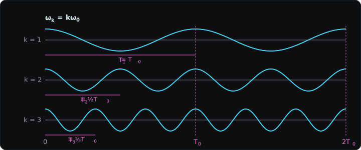
For a fundamental radian frequency $\omega_0$, the $k$th harmonic¹⁵ is the sinusoid whose radian frequency is $k\omega_0$. $k$ is the harmonic number and starts at 1.

$$ \omega_k = k\,\omega_0, \qquad f_k = k f_0, \qquad T_k = \frac{2\pi}{k\,\omega_0} = \frac{T_0}{k} $$

With $\omega_0 = 2\pi$ the first, second, and third harmonics have radian frequencies $2\pi$, $4\pi$, $6\pi$ and periods $1$, $\tfrac{1}{2}$, $\tfrac{1}{3}$ s. In the figure below, a larger $k$ oscillates $k$ times within the same $T_0$, and all three curves return to their starting point together at $t = T_0$. This is why the fundamental period of any sum of harmonics is $T_0$.

To decide whether a sum of sinusoids is periodic and to find its fundamental period, look only at the radian frequencies. The fundamental radian frequency of the sum is the greatest common divisor¹⁶ of the radian frequencies of the terms, and the harmonic number of each term is its radian frequency divided by $\omega_0$.

$$ x(t) = \cos(4\pi t) + \sin(6\pi t): \quad \omega_0 = 2\pi, \quad T_0 = 1 \text{ s}, \quad k = 2, 3 $$

If the ratio of the radian frequencies is irrational, no greatest common divisor exists and the sum is aperiodic.

Harmonically related complex exponentials

Writing the harmonics as complex exponentials¹⁷ instead of sinusoids gives the following set.

$$ \phi_k(t) = e^{\,jk\omega_0 t}, \qquad k = 0, \pm 1, \pm 2, \dots $$

For $k \neq 0$ the signal is periodic with radian frequency $|k|\omega_0$ and fundamental period $\tfrac{2\pi}{|k|\omega_0}$. The absolute value keeps the frequency and period positive when $k$ is negative, and for positive $k$ the expression matches the harmonic formulas. Every $\phi_k(t)$ has $T_0 = \tfrac{2\pi}{\omega_0}$ as a common period. For $k = 0$¹⁸, $\phi_0(t) = 1$ is a constant and no period is defined.

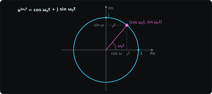
Euler’s formula splits the exponential into real and imaginary parts, which places it as a point on the complex plane (real part horizontal, imaginary part vertical).

$$ e^{\,j\omega_0 t} = \cos\omega_0 t + j\sin\omega_0 t $$

The point at time $t$ is $(\cos\omega_0 t, \sin\omega_0 t)$ with magnitude $\sqrt{\cos^2 + \sin^2} = 1$. It starts at $(1, 0)$ when $t = 0$, moves counterclockwise as $t$ increases, and returns to the start when $\omega_0 t = 2\pi$. Since it lies on the unit circle of radius 1 at every $t$, in polar form it has magnitude 1 and angle $\omega_0 t$.

Exercise 2

For $x(t) = 2\cos(6\pi t) + \sin(9\pi t)$, find the following.

(a) The fundamental radian frequency $\omega_0$ and fundamental period $T_0$ (b) The harmonic number of each term (c) The radian frequency $\omega_1$ and period $T_1$ of the first harmonic

Solution. The greatest common divisor of $6\pi$ and $9\pi$ is $3\pi$, so $\omega_0 = 3\pi$ rad/s and $T_0 = \tfrac{2\pi}{3\pi} = \tfrac{2}{3}$ s. Since $\tfrac{6\pi}{3\pi} = 2$ and $\tfrac{9\pi}{3\pi} = 3$, $2\cos(6\pi t)$ is the second harmonic and $\sin(9\pi t)$ is the third. The first harmonic has $\omega_1 = \omega_0 = 3\pi$ rad/s and $T_1 = T_0 = \tfrac{2}{3}$ s.